Sometimes, we may wanna simulate certain random variable to get the desired approximation. Yet, if the scenario is rather complicated, the computation cost can be exorbitant. With the help of inverse transformation method, we are able to generate many special random variables efficienctly.
A Toy Example
With replacement, we draw cards at random from an ordinary deck of 52 cards, and successively until an ACE is drawn. What is the probability of exactly 10 draws?
Apparently, let \(X\) be the number of draws until the first ace. The random variable \(X\) is of geometric distribution with the parameter \(p = \frac{1}{13}\). The answer of the desired probability is
\[ P(x) = (1-p)^{x-1} * p = (\frac{12}{13})^9 * (\frac{1}{13}) \]
Simulating \(X\)
Now, if we wanna approximate the desired probability by simulating \(X\), an intuitive way might look like as below:
1 | ### Pseudo-code of Simulation |
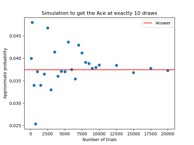
From the experiment, it can be observed that \(N\) has to be quite large (>10000) if we would like to get enough accuracy:

Below is the source code:
1 | import numpy as np |
However, this approach is not efficient because the time complexity is proportional to the draw number. Thus, let's introduce the inverse transformation method. By this method, we are able to get the same result as well but only need to choose one random point in (0,1), significantly reducing the time cost.
Inverse Transformation Method
Let \(F(X) = P(X \leq x)\) be the probability distribution function of the random variable \(X\). Remember that for uniform random variable \(U\) over \((0,1)\),
\[ F(U) = P(U \leq x) = x, x \in (0,1) \tag{1} \]
Imagine that our objective is to simulate a random variable \(X\) from a uniform random variable \(U\), i.e., \(P(X \leq x) = P(T(U) \leq x)\). We hope to find a transformation \(T\) that is able to convert the random variable \(U\) into our desired \(X\).
$$ \displaylines { P(X \leq x) \\ = P(T(U) \leq x) \\ = P(U \leq T^{-1}(x)) \\ } $$Remember that \(F(X) = P(X \leq x)\) and from \((1)\):
$$ \displaylines { P(U \leq T^{-1}(x)) \\ = P(U \leq F(x)) \\ = P(F^{-1}(U) \leq x) } $$\[ \longrightarrow X = F^{-1}(U) \tag{2} \]
From \((2)\), we know the transformation \(T\) we are looking for is just \(F^{-1}\). Therefore, after solving \(F^{-1}\), we are able to generate the desired \(X\) from uniform random variable \(U\) directly without complications.1
Simulating Geometric Distribution via Inverse Transformation Method
Back to our original problem, we wanna simulate \(X\) in the toy example, and we know that the \(F(x)\) of geometric distribution with parameter \(p\) is
\[ F(x) = 1 - (1-p)^{x-1} \]
Solve \(u = F(x)\):
$$ \displaylines { u = 1 - (1-p)^{x-1} \\ x = 1 + \frac{\log{(1-u)}}{\log{(1-p)}} } $$\[ \equiv 1 + \frac{\log{u}}{\log{(1-p)}} \tag{3} \]
If \(u\) is a random number variable from (0,1), then \((1-u)\) is a random number variable from (0,1) as well.
Now, from \((3)\), we are able to generate \(X\) from \(U\) efficiently. Because \(X\) is an integer, we use the floor operation (with the ceiling is also equivalent):
\[ X = \lfloor 1 + \frac{\log{u}}{\log{(1-p)}} \rfloor \]
1 | ### Pseudo-code of Geometric Distribution Simulation with Inverse Transform method |
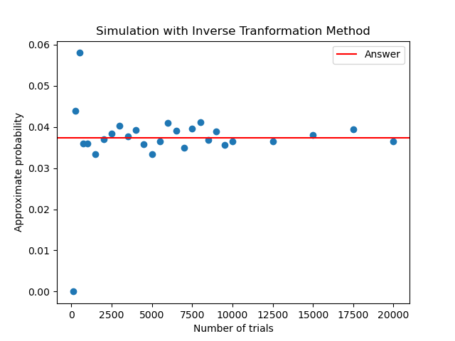
Below is the experimental result and the related source code:

1 | import numpy as np |
Performance Comparison
Let N be 500000 trials.
Original method:
1 | ### Original Method |
Inverse transformation method:
1 | from time import perf_counter |
Results:
| N = 500000 (trials) | Elapsed Time (sec) |
|---|---|
| Original Method | 10.832 |
| Inverse Transformation Method | 0.363 |
We can observe that the elapsed time has been substantially reduced after applying inverse transformation method.
Note that the inverse transformation method is to mainly improve the computation cost. It does not increase the convergence rate. From the previous experimental results, you can see that the N trials required to converge are roughly the same for both methods.
For rigorous proof, you can refer to Inverse transform sampling. The aim here is to grasp the idea intuitively.↩︎