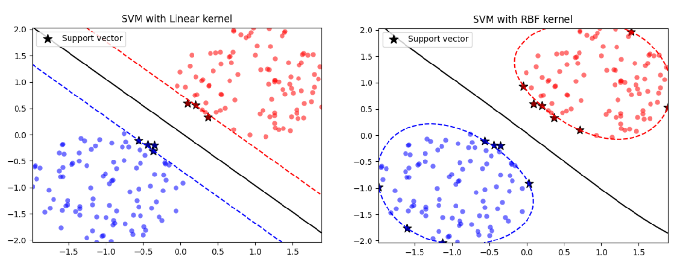
Support vector machine (SVM) plays an important role in machine learning. Actually, SVM is one of my favorite models because of its analytical property. Its main idea is to find the optimal hyperplane that can linearly separate the data, or maximise margin in the feature space. It is one of the most robust models based on statistical learning framework in VC theory (Vapnik–Chervonenkis theory). The determination of the model parameters is a quadratic programming problem, or convex optimisation more specifically. Its solution is usually sparse, and the new input prediction depends only on the evaluation of a subset of training data with kernel function. One of the most common and efficient approaches to train SVM is sequential minimal optimisation (SMO), which breaks down the problem into solving a pair of parameters analytically at each step. Besides, SMO also eliminates the need for matrix storage issue when the training data size is huge.
Recall the Objective Function of SVM
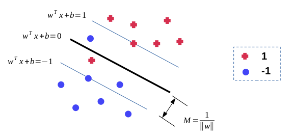
We want to find a hyperplane \(w^T x + b = 0\) and maximise the margin width \(2M\) in order to separate the data labeled as \(y = \pm 1\). All data points should be correctly classified, i.e. \(y_i(w^T x_i + b) > 0\) for all \(i\),
$$ \displaylines { \max_{w,b} M \\ \textrm{ s.t. } \frac{y_i(w^T x_i + b)}{ \Vert w \Vert} \ge M, \forall i=1,2,...,N } $$The above optimisation problem can be converted into a dual form of Lagrangian function, maximising \(L\):
$$ \displaylines { L(\alpha)=\sum^{N}_{i} \alpha_i - \frac{1}{2} \sum^{N}_{i}\sum^{N}_{j} y_i y_j \alpha_i \alpha_j {x_i}^T x_j \\ \textrm{ s.t. } 0 \le \alpha_i, \forall i \\ \textrm{ and } \sum^{N}_{i}y_i \alpha_i = 0 } \tag{1} $$The solution for \(w\) is
\[ w = \sum^{N}_{i} y_i \alpha_i x_i \tag{2} \]
If we allow some points are misclassified with penalty \(C\), then the constraints of \(\alpha_i\) become
\[ 0 \le \alpha_i \le C, \forall i \]
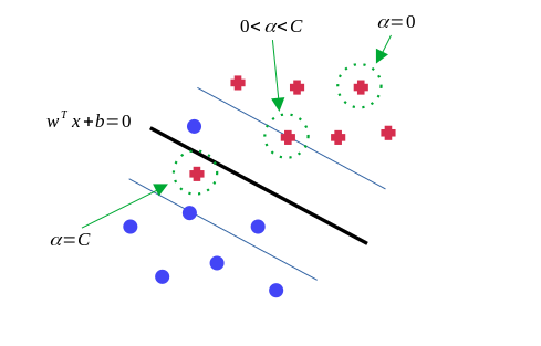
For points with \(0 \lt \alpha_i \lt C\), they just lie on the edge of the margin. In contrast, when \(\alpha_i = 0\), it is in the decision boundary and does not contribute to the prediction. The points with \(\alpha_i = C\) lie inside the margin and might either be classified correctly or not.
Points with non-zero \(\alpha_i\) are called support vectors. These can be demonstrated as below:
If we apply the feature transformation with kernel function \(K(x_i, x_j)\), then the Lagrangian function \((1)\) turns into
\[ L(\alpha)=\sum^{N}_{i} \alpha_i - \frac{1}{2} \sum^{N}_{i}\sum^{N}_{j} y_i y_j \alpha_i \alpha_j K(x_i, x_j) \tag{3} \]
The constraints of Lagrangian multipliers are the same as before.
The predicted \(\hat{y}\) of new input is
\[ \hat{y} = \sum^{N}_{i} y_i \alpha_i K(x_i, x) + b \tag{4} \]
Sequential Minimal Optimisation
SMO process mainly contains two parts: one is to solve two Lagrangian parameters analytically at a step, and then decide how to choose these two parameters heuristically for speed up.
Solving Lagrangian Multipliers
Using the constraint \(\sum^{N}_{i}y_i \alpha_i = 0\) in \((1)\), we can get
\[ 0 = y_1 \alpha^{old}_1 + y_2 \alpha^{old}_2 + \sum^{N}_{i=3}y_i \alpha_i = y_1 \alpha^{new}_1 + y_2 \alpha^{new}_2 + \sum^{N}_{i=3}y_i \alpha_i \]
\[ \Rightarrow y_1 \alpha^{old}_1 + y_2 \alpha^{old}_2 = k = y_1 \alpha^{new}_1 + y_2 \alpha^{new}_2 \tag{5} \]
where \(k = -\sum^{N}_{i=3}y_i \alpha_i\).
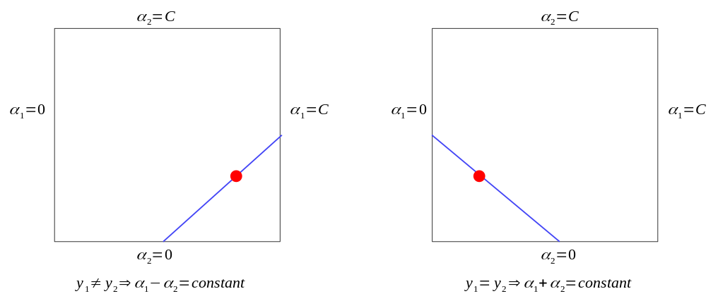
Remember that \(y\) is either \(1\) or \(-1\) , with the constraint \(0 \le \alpha_i \le C\), \(\alpha_1\) and \(\alpha_2\) can only lie on the diagonal line segment shown as below:
The Lagrangian multiplier \(\alpha_2\) can be solved by the first derivative of the objective function to find its extremum. The analytical form to solve \(\alpha_2\) is
\[ \alpha^{new}_2 = \alpha^{old}_2 + y_2 \frac{E_2 - E_1}{\eta}, \]
\[ E_i = \hat{y_i} - y_i \text{, } \eta = K_{11} + K_{22} - 2K_{12} \tag{6} \] \[ K_{ij} = K(x_i, x_j) \]
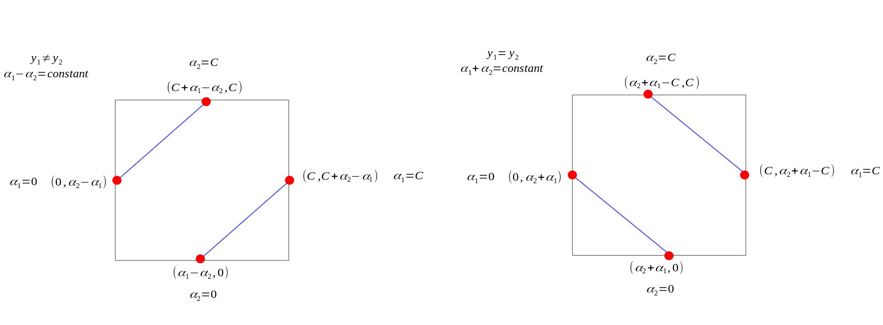
Case 1: \(y_1\) \(\neq\) \(y_2\)
\[ L = \max(0, \alpha_2 - \alpha_1) \]
\[ H = \min(C, C + \alpha_2 - \alpha_1) \]
Case 2: \(y_1 = y_2\)
\[ L = \max(0, \alpha_2 + \alpha_1 - C) \]
\[ H = \min(C, \alpha_2 + \alpha_1) \]
The \(\alpha^{new}_2\) should be bounded by \(L\) and \(H\).
$$ \alpha^{new}_2=\begin{cases} L, & \text{if $\alpha^{new}_2 \lt L$}.\\ \alpha^{new}_2, & \text{if $L \le \alpha^{new}_2 \le H$}.\\ H, & \text{if $\alpha^{new}_2 \gt H$} \end{cases} $$We can then obtain \(\alpha^{new}_1\) by multiplying \(y_1\) on both sides in \((5)\),
\[ \alpha^{new}_1 = \alpha^{old}_1 + y_1 y_2 (\alpha^{old}_2 - \alpha^{new}_2) \tag{7} \]
Abnormal Case for \(\eta\)
Normally, \(\eta\) should be greater than 0. However, if we encounter the abnormal case that \(\eta \le 0\), e.g. picking the same points or an incorrect kernel that does not obey Mercer's condition, the full version of SMO algorithm will move the Lagrangian multiplier to the end of the line segment that can maximise the objective function.1 2
Another simple way to handle this is to treat the scenario as no progress being made for this pair of \(\alpha\).
Comupting the Threshold b
We can update the threshold \(b\) after getting \(\alpha\) at each step.
When \(0 \lt \alpha_1 \lt C\), \(b_1\) is a valid threshold because it makes the output \(\hat{y_1}\) be the same as \(y_1\) when the input is \(x_1\)
\[ E_1 = (y_1 \alpha^{old}_1 K_{11} + y_2 \alpha^{old}_2 K_{12} + b) - (y_1 \alpha^{new}_1 K_{11} + y_2 \alpha^{new}_2 K_{12} + b_1) \]
\[ \Rightarrow b_1 = b - E_1 - y_1 (\alpha^{new}_1 - \alpha^{old}_1) K_{11} - y_2 (\alpha^{new}_2 - \alpha^{old}_2) K_{12} \]
Similarly, when \(\alpha_2\) is not at bounds, \(b_2\) is a valid threshold
\[ b_2 = b - E_2 - y_1 (\alpha^{new}_1 - \alpha^{old}_1) K_{12} - y_2 (\alpha^{new}_2 - \alpha^{old}_2) K_{22} \]
When both \(b_1\) and \(b_2\) are valid, they will be equal because \(\hat{y_i} y_i = 1\), and the new \(E_1\) and \(E_2\) will be 0. This can be easily verified with \((6)\) and \((7)\). Intuitively, when \(y_1 = y_2\), they are both at bounds and is trivial, whereas for \(y_1 \neq y_2\), they both try to maximise the margin width, and this results in \(b_1\) and \(b_2\) being equal.
For other cases, we could choose the halfway between \(b_1\) and \(b_2\).
$$ b=\begin{cases} b_1, & \text{if $0 \lt \alpha^{new}_1 \lt C$}.\\ b_2, & \text{if $0 \lt \alpha^{new}_2 \lt C$}.\\ \frac{(b_1+b_2)}{2}, & \text{otherwise}. \end{cases} $$Choosing the Multipliers to Optimise
In order to speed up the training rate, the main idea of choosing the multipliers in SMO can be briefly summarised as the following.
Firstly, choose the multiplier that are likely to violate the KKT conditions to optimise, i.e. \(0 < \alpha_i < C\). When one multiplier is chosen, another multiplier would be the one that can maximise the step size, \(\vert E_2 - E_1 \vert\).
Then SMO will scan the entire data sets until the algorithm terminates.
Other Tricks to Make the Training Process Faster
Error Cache Update
We can reduce the computational cost to compute the error cache, which stores \(E_i\), after Lagrangian multipliers update. From \((6)\),
\[ E^{old}_i = y_1 \alpha^{old}_1 K_{1i} + y_2 \alpha^{old} K_{2i} + \sum^N_{j=3} y_j \alpha_j K_{ij} + b - y_i \]
\[ E^{new}_i = y_1 \alpha^{new}_1 K_{1i} + y_2 \alpha^{new} K_{2i} + \sum^N_{j=3} y_j \alpha_j K_{ij} + b_{new} - y_i \]
\[ \Rightarrow E^{new}_i = E^{old}_i + y_1 (\alpha^{new}_1 - \alpha^{old}_1) K_{1i} + y_2 (\alpha^{new}_2 - \alpha^{old}_2) K_{2i} + (b_{new} - b) \]
Linear SVM Optimisation
The linear SVM only needs to store a single weight vector, \(w\). It can also be updated using similar mechanism as error cache. From \((2)\),
\[ w^{old} = y_1 \alpha^{old}_1 x_1 + y_2 \alpha^{old}_2 x_2 + \sum^N_{j=3} \alpha_j x_j \]
\[ w^{new} = y_1 \alpha^{new}_1 x_1 + y_2 \alpha^{new}_2 x_2 + \sum^N_{j=3} \alpha_j x_j \]
\[ \Rightarrow w^{new} = w^{old} + y_1 (\alpha^{new}_1 - \alpha^{old}_1) x_1 + y_2 (\alpha^{new}_2 - \alpha^{old}_2) x_2 \]
Implementation
Source Code
1 | # File: MySVM.py |
Demo
1 | # File: SVM_test.py |
